To create charts in Excel, put your labels and numbers in a small table, select the data, and open Insert → Recommended Charts. Choose a chart that makes the comparison easy to understand. This guide uses a simple column chart to compare study time across five days.
You will build the chart, label it, change a value, and check that the result updates. The example uses fictional data and ordinary Excel features. Menu names can differ between Windows, Mac, and Excel for the web; the main steps stay the same.
Download the free Excel chart practice file
Download the Excel chart practice workbook (.xlsx). It contains one worksheet, five editable study-time values, an editable column chart, and formulas for the total and daily average. You can also build the example from a blank workbook using the steps below.
1. Prepare the data for your Excel chart
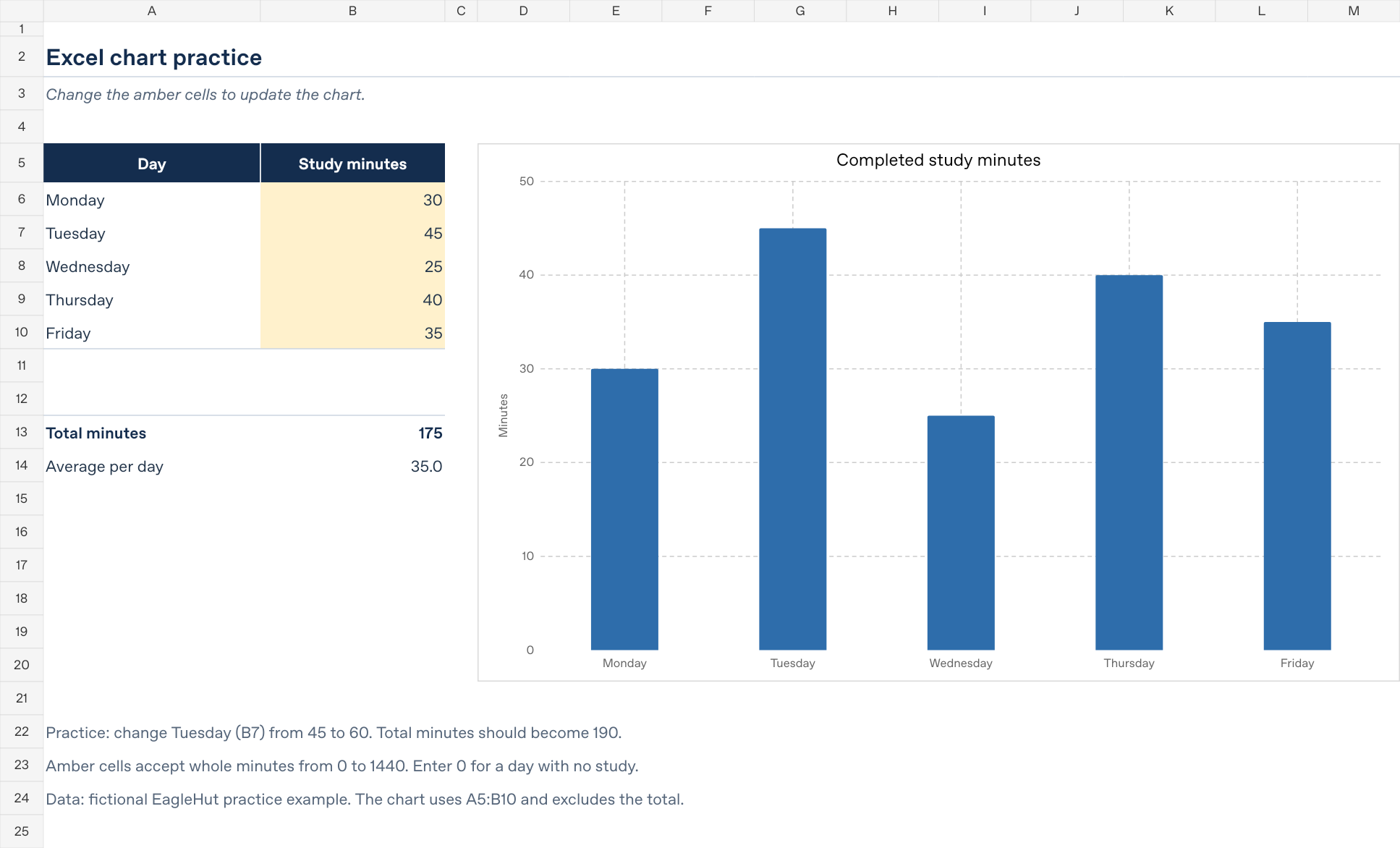
In the download, open the Chart practice worksheet. If you are starting from a blank workbook, enter this table in A5:B10. Row 5 contains the headings, and rows 6–10 contain the five days.
| Day | Study minutes |
|---|---|
| Monday | 30 |
| Tuesday | 45 |
| Wednesday | 25 |
| Thursday | 40 |
| Friday | 35 |
Keep the day names in column A and the numbers in column B. Enter 30, rather than “30 minutes”, in the numeric cell. The heading supplies the unit. Use the same unit for every row, and keep empty spacer rows outside the selected table.
For this exercise, Tuesday should be the highest value at 45 minutes and Wednesday the lowest at 25 minutes. Those two checks will help you catch a wrong selection later.
2. Create a column chart in Excel
- Select A5:B10, including both headings and all five data rows.
- Open Insert → Recommended Charts.
- Choose a 2-D Clustered Column chart. If it is not recommended, look under All Charts → Column. Some versions also offer column charts directly on the Insert tab.
- Insert the chart and move it beside the table so both remain visible.
You should see five vertical columns, with Monday through Friday along the bottom. The heights should match the numbers in the table. Leave the Total minutes and Average per day rows out of the chart selection: they summarize the same data and would add misleading extra columns.
3. Add a clear title and readable labels
Change the chart title to Completed study minutes. Label the vertical value axis Minutes. On Windows, chart elements are available under Chart Design → Add Chart Element; other editions may show them in a chart formatting pane.
- Use one color for this single series so the column heights carry the comparison.
- Keep zero visible on the vertical axis. Cutting off the bottom of columns can exaggerate a small difference.
- Keep the day labels readable. A simple 2-D chart is enough for this example.
- A legend is optional here because the title and axis already identify the one series.
4. Change a value and check that the chart updates
In the practice file, change Tuesday in B7 from 45 to 60. Its column should become taller. The total should change from 175 to 190 minutes, and the daily average should change from 35 to 38 minutes. Change B7 back to 45 to restore the original example.
The total in B13 uses =SUM(B6:B10). The average in B14 uses =AVERAGE(B6:B10). These formulas summarize the five numeric cells; the chart reads those source cells directly. You do not need a formula merely to insert a chart.
For a second check, restore Tuesday to 45, then change Monday from 30 to 50. The total should become 195 minutes and the average 39 minutes. Restore Monday to 30 when you finish.
5. Fix common Excel chart problems
| What you see | What to check |
|---|---|
| A day is missing | Check that the selected source includes every intended row. If you add Saturday below the table, extend the chart source to include it. |
| The total appears as another column | Reselect only A5:B10. Keep summary rows outside the chart data. |
| The day names appear as separate series | Check the selected range and use Chart Design → Switch Row/Column when the orientation is wrong. |
| A value is missing or treated as text | Re-enter it as a plain number in the source cell. Changing only the display format does not always convert stored text. |
| Editing a number does not change the picture | Make sure you are editing the original Excel chart and its source range. A copied screenshot is a static image. |
If you expand the table, also update any total and average formulas to cover the extra rows. Extending the chart range alone does not extend every separate formula in the workbook.
Which Excel chart type should you choose?
- Column chart: useful for comparing a small set of category values, as in this five-day example.
- Line chart: useful when the main question is how values change over an ordered timeline. Keep the dates in order.
- Horizontal bar chart: useful when category names are long and need more room.
Choose the chart around the question you want to answer. A chart comparing minutes should keep minutes as its unit; avoid mixing a count, a percentage, and a duration on one unexplained axis.
Continue practising
Try the same method with a small table of fictional spending, books read, or tasks completed. Name the units, keep the source data beside the chart, and check the tallest and shortest values before sharing it.
For another beginner exercise, follow Create a Weekly Study Planner in Excel or Build Your First Spreadsheet Budget.